Usage distribution
How time is spread across applications, categories, and hours of day.
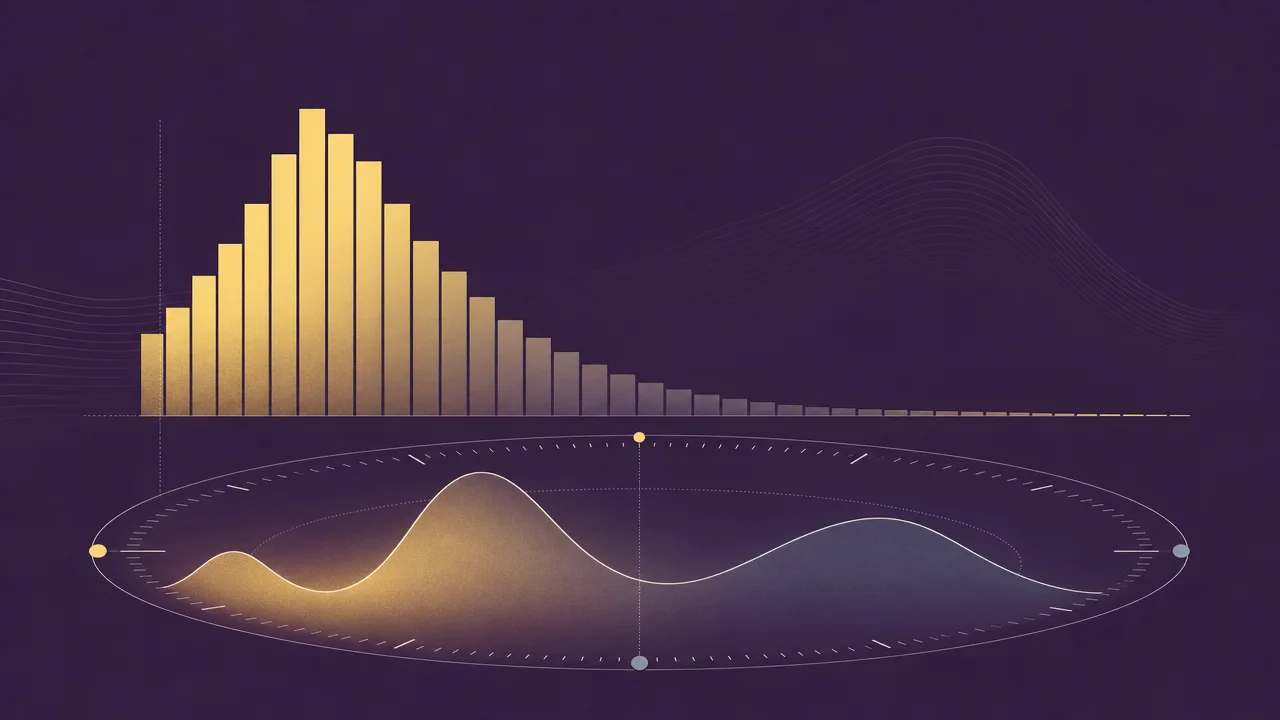
Usage distribution describes the shape of computer time. Where active time tells you how long a person was present at the keyboard, and application usage tells you which programs they touched, usage distribution captures how that time was allocated across everything they did. It is the answer to questions like whether a day was concentrated in one or two tools, scattered across dozens, or skewed toward a particular part of the morning.
This page covers what usage distribution is, why its shape matters, the techniques people use to read it, the common patterns that show up in knowledge work, and the misconceptions that grow up around it.
What is usage distribution?
Usage distribution is the statistical shape of how computer-usage time is spread out. It can be sliced along several axes: by application, by application category, by website, by project, and by hour of day. In each case the underlying question is the same. Once total time is broken into smaller pieces, how are those pieces sized, and how are they arranged.
A distribution by application answers questions like which program dominates the day, how quickly the time falls off after the top few, and how many programs receive only a token amount of attention. A distribution by category groups those programs into bands such as development, communication, design, or entertainment, and shows the balance between them. A distribution by hour of day shows when activity actually happens, and where the quiet stretches sit.
None of these shapes are a single number. They are descriptions, usually rendered as charts. Reading them well is closer to reading a fingerprint than to checking a thermometer, which is why the most useful analytics tools spend more effort on the visualisation than on the totals.
Why does usage distribution matter?
A daily total of active time gives a coarse summary. The same total can sit behind a deep, focused day in two applications or a fragmented day across thirty. Usage distribution makes that difference visible. Two people who both spent six hours on the computer can have completely different working patterns, and the shape of the distribution is what shows it.
For individuals, the distribution is often where the most actionable information lives. A long tail of small sessions tends to correlate with switching and interruption. A heavy concentration in a single tool, paired with the right kind of tool, is a sign of sustained attention. The hour-of-day shape reveals whether the day matches a personal energy curve or fights against it.
For teams, distributions show how tools are actually being used rather than how they were intended to be used. An application meant to be central that lives in the long tail of most users is a useful signal. A category such as communication that quietly dominates the working day is another. These patterns are easier to read in shape than in a list of totals.
How is usage distribution analysed?
Several views are useful, and each highlights a different part of the picture. None of them are exotic, and the more careful analytics tools use them in combination rather than picking a favourite.
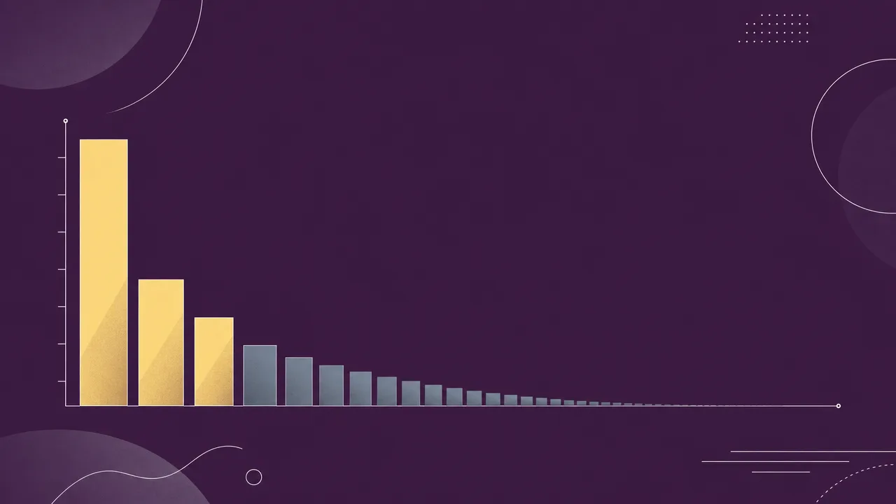
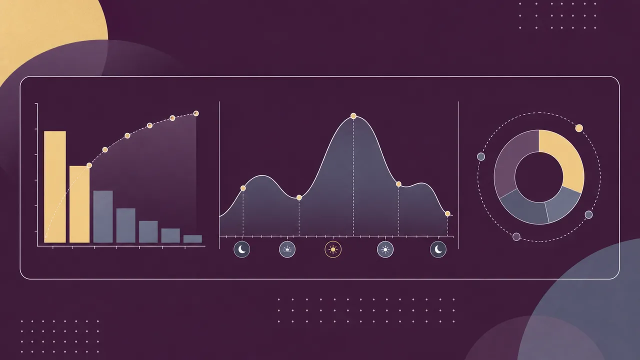
A histogram of time per application is the most common starting point. Sorted from largest to smallest, it shows the head of the distribution clearly and makes the long tail visible as a flat region to the right. The same view in cumulative form, where each bar adds onto the previous one, makes it easy to read off how many applications cover any given fraction of the day.
A Pareto chart applies the 80/20 lens explicitly. It ranks items from largest to smallest and overlays a cumulative curve, so the eye can see how few applications account for the bulk of the time. The pattern is not guaranteed in any one user's data, but it is common enough to be a useful reference. The principle itself goes back to Vilfredo Pareto in 1896 and has been observed in many software-usage contexts, including feature usage and crash sources, where a small fraction of items often accounts for a large fraction of the total.
A category pie or stacked bar groups applications into bands such as software development, communication and scheduling, design, reference and learning, social, and entertainment. RescueTime, for instance, organises activities into eleven main categories and sixty-four sub-categories, and the resulting bands give a readable summary of the day at a higher level than individual application names.
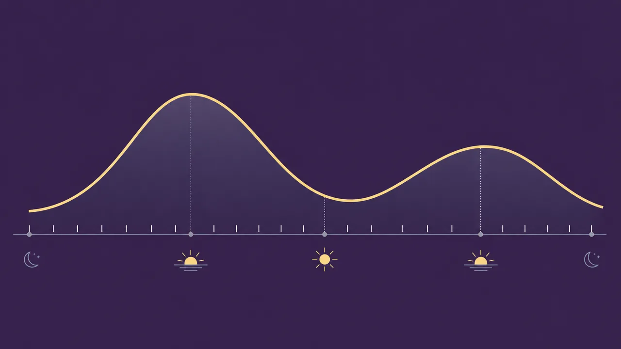
A time-of-day curve, often called an activity curve or an hour-of-day histogram, plots active time against the hours of the day. It shows when work actually happens, where the quiet stretches sit, and whether the shape repeats across days of the week. Heatmaps that combine day of week with hour of day make the weekly pattern visible at a glance.
Concentration indices summarise the shape into a single number. The most common is the share of time taken by the top one, three, or five applications. Researchers sometimes borrow tools from economics, such as the Gini coefficient, to compare distributions across people or weeks. These numbers are useful for tracking change over time, but they hide the underlying pattern and should always be read alongside the chart.
Common benchmarks
Reliable population benchmarks for usage distribution are sparse, and most of the cleanly published numbers describe related metrics rather than distribution shape directly. The patterns below are widely reported, but individual variation is the rule rather than the exception.
- Pareto-shaped distributions are common in software-feature use and application time. Microsoft has reported that a small fraction of code paths accounts for a large fraction of crashes, and similar imbalances appear in which applications dominate a working day. Whether a given user shows an 80/20 split exactly is an empirical question, not a rule.
- Daniel Pink's review of chronobiology research in When (2018) reports that roughly 80 percent of people experience a peak early in the day, a trough in the early to mid afternoon, and a partial recovery in the evening. The trough typically lands about seven to eight hours after waking, often between 14:00 and 16:00 for standard schedules.
- Microsoft's Work Trend Index has consistently described the working day as fragmented across meetings, communication, and focused work, with the precise category mix varying year to year. The general pattern of communication time taking a large share of the day is robust across reports.
- Long-tail patterns in application use are widespread enough that long-tail analysis is a standard practice in software-asset management, where a few applications cover most of the spend and use while a large set of smaller tools accounts for the remainder.
These figures should be read as orientation rather than as targets. For an individual, the more useful comparison is almost always the same person's own distribution over time.

Examples
Three short scenarios show how the same total time can hide very different distributions.
A backend engineer ends the day with six hours of active time. The distribution by application is steep: the code editor takes about three hours, the terminal about an hour and a half, and the browser another hour. A long tail of small items, including a chat client, a calendar, and a music player, covers the remaining thirty minutes. The hour-of-day curve shows a strong morning peak, a soft afternoon dip, and a second peak after the afternoon stand-up.
A product manager hits the same six-hour total but with a very different shape. No single application crosses an hour. A spreadsheet, a chat client, a video-call window, a document editor, and a project tracker each take roughly the same amount of time, with a long tail of browser tabs underneath. The hour-of-day curve is flat across the day, with no clear peak. The total is identical to the engineer's, but the experience of the day is not.
A student spends four hours of active time on the computer. The distribution by category is concentrated: about 75 percent in reference and writing tools, 15 percent in reference and learning, and 10 percent in a social application. The hour-of-day curve has a clear gap in the middle of the afternoon and a long evening tail that runs past 22:00. The shape is consistent with a chronotype that prefers later work, and the concentration is consistent with focused study.
Misconceptions
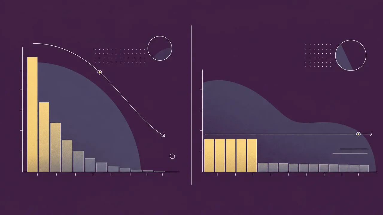
The most common misconception is that a long tail is a problem in itself. A long tail is just the mathematical signature of many small contributors, and small contributors are not automatically bad. A developer may briefly touch a dozen utilities in a single hour without losing focus. The tail becomes a problem when it is full of unintended switches, not when it is simply present.
A second misconception is that a concentrated distribution is always a sign of good work. Concentration in a single editor for hours is consistent with deep work. The same concentration in a feed reader or a video site is consistent with the opposite. The shape carries no judgement about the content, and any reading of it should be paired with what the dominant applications actually are.
A third misconception is that an averaged distribution is representative. Workdays, meeting days, deep-work days, and weekends usually produce different shapes. Averaging them together blurs the patterns and can hide both healthy and unhealthy behaviour. Per-day, per-weekday, or per-project views almost always carry more information than a single all-time chart.
A fourth, subtler misconception is that the hour-of-day curve reflects ambition. It largely reflects chronotype, schedule, and the structure of the workday. Trying to force a different curve without changing the schedule rarely sticks.
Related concepts
Usage distribution sits between raw activity data and the higher-level metrics built on top of it. Understanding it well usually means being comfortable with several neighbouring ideas.
- Application usage: the per-program totals that the distribution is built from.
- Usage analytics: the broader practice of turning usage data into patterns and reports.
- Activity trends: how the distribution shifts over weeks, months, and seasons.
- Foreground application: the program that owns the time at any moment, and the basis for attribution.
- Productivity metrics: classifications of categories that turn a distribution into a productive-versus-distracting view.
- Active time: the underlying duration the distribution allocates.
- Focus time: sustained, single-application stretches that often sit at the head of a concentrated distribution.
- Context switching: the behaviour that produces a long tail and a flat hour-of-day curve.
- Workday fragmentation: a high-level description of distributions that are scattered across applications and hours.
- Application switching: the moment-to-moment behaviour that shapes the tail of the distribution.
Tracking usage distribution
Usage distribution can be tracked by any tool that records active time against the foreground application and retains enough history to build a shape from. The mechanics are not complicated: each second of input is attributed to whichever window owns it, the totals are aggregated per application and per hour, and the charts are built from those aggregates. The difference between tools lies less in the recording and more in how the resulting shape is presented.
WhatPulse runs locally on Windows, macOS, and Linux and stores per-application and per-time-window data on the device by default. That makes it straightforward to look at the head and tail of the distribution, to compare days and weekdays, and to see the hour-of-day curve without sending raw data anywhere. Users who enable optional sync gain longer-term trend views, which is where distribution analysis tends to be most useful, since a single day is rarely representative.
The reason for measuring distribution is not to enforce a particular shape. It is to make the shape visible enough to recognise. Once the pattern is visible, decisions about which applications to defend, which to trim, and how to schedule the day can be made deliberately rather than by guesswork.
Frequently asked questions
Is a concentrated usage distribution good or bad?
Neither on its own. Concentration on a code editor for a developer or a writing application for an author is a healthy sign of focus. The same concentration on a social feed is the opposite. The shape only carries meaning once paired with what the dominant applications are.
What is the difference between usage distribution and application usage?
Application usage reports the time spent in each program. Usage distribution describes the overall shape of those numbers, including how steeply they fall off, how many applications cover most of the day, and how the time spreads across the hours of the day.
Does the Pareto principle really apply to computer use?
Often, but not as a law. Vilfredo Pareto observed the 80/20 pattern in 1896 in wealth distribution, and similar imbalances are common in software feature use and application time. Whether any one user fits the pattern is an empirical question, not a guarantee.
Why does my usage distribution look different on different days?
Workdays, meeting days, deep-work days, and weekends usually produce very different shapes. Averaging them together can hide that variation. Looking at distributions per weekday or per project tends to be more informative than a single all-time chart.
What is a long tail in usage distribution?
It is the set of applications you use briefly or rarely. Even when each one accounts for only a few minutes, together they can represent a meaningful share of the day, and they are often where unplanned context switching hides.
When during the day are most people active on their computers?
Research summarised by Daniel Pink in When (2018) suggests roughly 80 percent of people show a peak in the morning, a trough in the early to mid afternoon, and a partial recovery later. The exact times shift with chronotype, but the general shape is widespread.
Can usage distribution measure productivity?
Indirectly. It can show whether attention is concentrated or scattered and whether time is going to productive categories, but it does not measure output. It is best read alongside focus time and the productivity classification of the categories involved.
How many applications do most knowledge workers use in a day?
This varies widely by role. Long-tail patterns are common, with a handful of applications dominating the time and a much longer list contributing a few minutes each. Specific averages depend on the dataset and should be treated as approximate.
Conclusion
Usage distribution is the shape behind the totals. It describes how computer time is spread across applications, categories, and hours of the day, and it carries information that a single number cannot. Read well, it shows whether a day was focused or scattered, whether the schedule matched a personal energy curve, and where the quiet attention drains live.
Like most measurement, it is most useful when treated as a description rather than a verdict. The shape says what happened. Whether the shape is the right one is a question for the person reading it, in light of what they were trying to do that day.